Different Methods to Treat Outliers of Datasets with Python Pandas

Practical methods helping you treat outliers during data processing step of data analysis

In the last article, we used different method to detect the outliers in the datasets. In this article, we will learn how to treat outliers using some convenient methods in the Pandas library.

This article is the Part VII of Data Analysis Series, which includes the following parts. I suggest you read from the first part so that you can better understand the whole process.

Table of Contents

1. Preparation to Start

(1) import required packages

import numpy as np
import pandas as pd

(2) read data

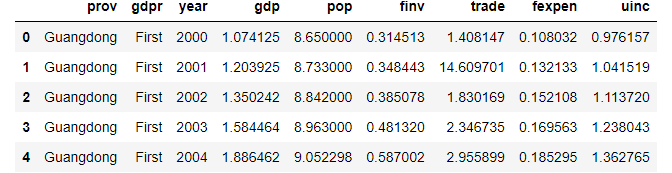
We use the dataset that we have stored after imputing the missing values of the original dataset in the article of imputing missing values.

# read data
df = pd.read_csv('./data/gdp_china_mis_filled.csv')

# display the first 5 rows
df.head()

2. Remove the outliers

(1) quantile range method

In the last chapter, we have found trade column has two outliers through different outlier detection methods, and quantile range method is one of these methods.

Here, the outliers-removed method is to remove the outliers’ rows from the data. First, we use the thresholds defined in the last article.

# create thresholds
min_threshold, max_threshold = df['trade'].quantile([0.01,0.99])

# create a new dataframe excluding the outlier rows
outlier_removed = df[(df['trade'] < max_threshold)&(df['trade'] > min_threshold)]

# diplay the shape of new dataset
print(outlier_removed.shape)

# the orignal shape 
print(df.shape)

The original dataframe has 95 rows, but the new dataframe is only 93, indicating that the two outliers’ rows have been deleted.

(2) use `drop()` method

outlier_removed2 =df.drop([1,93])

# print the shape
outlier_removed2.shape

3. Regard outliers as NaNs

The process of this method is to replace the outliers with NaN, and then use the methods of imputing missing values that we learned in the previous chapter.

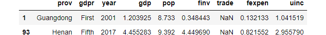
(1) Replace outliers with NaN

# change the outliers with 'np.nan'
df.loc[[1,93],['trade']]=np.nan
df.loc[[1,93]]

(2) Apply methods of missing values imputation

We can use any methods to impute missing values introduced in the last chapter. We use cubic spline interpolation method in this example.

outlier_removed3 = df.interpolate(method='cubicspline',order=2)

# display the outlier rows
outlier_removed3.loc[[1,93]]

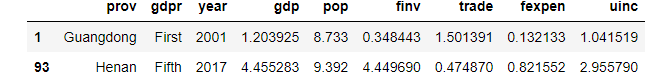
From the above output, we can see that the two outliers in trade have been replaced with 1.501391 and 0.474870.

4. Save the treated data

At the end, let’s save our processed dataset with an easy-recognized name, for example, into the local working directory gdp_china_outlier_treated.csv for further use in the future.

outlier_removed3.to_csv('./data/gdp_china_outlier_treated.csv',index=False)

5. Online Course

If you are interested in learning Python data analysis in details, you are welcome to enroll one of my course:

Master Python Data Analysis and Modelling Essentials

Bookmark

ClosePlease login

0 - 0

Thank You For Your Vote!

Sorry You have Already Voted!

Please follow and like me:

Different Methods to Treat Outliers of Datasets with Python Pandas