Practical Process to Develop Machine Learning Regression Models with Python

A real-world example to display the method to develop a machine learning regression model with Sckit-learn

The previous several posts displayed a general process to establish a classical statistic linear regression model. This article will investigate how to develop a linear regression models with machine learning approach using Scikit-learn, a machine learning library in Python.

We continue using the same preprocessed data used so that you can compare the results obtained from these two approaches.

Anaconda offers Scikit-learn as part of its free distribution. Otherwise, you can install it by:

pip install -U scikit-learn

In general, the process of developing a machine learning linear regression model should start from data preprocessing. Since we already preprocessed the dataset in previous posts, we start from importing required packages and reading this encoded dataset in this post.

1. Import required packages

We need the following packages, and we import them first.

import pandas as pd
import matplotlib.pyplot as plt
from sklearn.preprocessing import MinMaxScaler
from sklearn.model_selection import train_test_split
from sklearn.linear_model import LinearRegression
from sklearn.metrics import r2_score, mean_absolute_error,mean_squared_error,mean_absolute_percentage_error

2. Read data

In two of my previous posts, it displayed how to read data from GitHub depository and from Google Drive. Here I just read the dataset from my GitHub repository. If you are not familiar with these process, you can read the related posts.

url = 'https://raw.githubusercontent.com/shoukewei/data/main/data-pydm/gdp_china_encoded.csv'
df = pd.read_csv(url,index_col=False)
df.head()

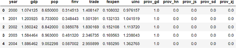
We have already discussed the notations of these variables, and correlation analysis showed strong linear relations between variables. This is why we will develop a linear regression model to predict GDP using the rest socio-economic factors.

3. Slice data into features X and target y

We divide the data into features X and target y, where gdp is target y and the rest variables are features X.

X = df.drop(['gdp'],axis=1)
y = df['gdp']

4. Split dataset for model training and testing

Then the features X and target y are further split into training dataset and testing dataset.

X_train, X_test, y_train, y_test = train_test_split(X, y,test_size=0.30, random_state=1)

5. Data Normalization

There are two previous posts on normalization methods and proper normalization process. In this case, we use MinMaxScaler method to normalize the data into the range of [0,1]. Please aware that proper process of data normalization is to (1) split training and testing data first, (2) training and testing data should use the same normalization scaler, (3) encoded string/categorical variable should not be normalized, etc. We have already normalized the dataset in these two previous posts, and I just copy it below. I suggest you reading these previous posts if you are not familiar with these points.

# MinMaxScaler method
# slice the continous features of training dataset
X_train_continuous = X_train.loc[:,'year':'uinc']
# fit the scaler and transform the training features
min_max_scaler = MinMaxScaler().fit(X_train_continuous)
X_train_continous_scaled = min_max_scaler.transform(X_train_continuous)
# get scaled X_train dataset
X_train_scaled = X_train.copy()
X_train_scaled.loc[:,'year':'uinc'] = X_train_continous_scaled

# slice the continous features of testing dataset
X_test_continuous = X_test.loc[:,'year':'uinc']
# transform the data
X_test_continous_scaled = min_max_scaler.transform(X_test_continuous)
# get scaled X_test dataset
X_test_scaled = X_test.copy()
X_test_scaled.loc[:,'year':'uinc'] = X_test_continous_scaled

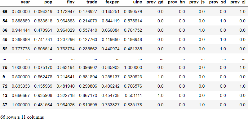
# display the scaled training dataset, for example
X_train_scaled

6. Train the model

Since the datasets have been prepared, we use the training data to train the model. It is very straightforward to define the linear regression model with LinearRegression() function in Scikit-learn, and fit the model using the training dataset with fit() function.

lr = LinearRegression()
model = lr.fit(X_train_scaled, y_train)

7. Evaluate the model

We can use predict() method to calculate the prediction values on training data and testing data.

(1) Training performance

To calculate the prediction values on training dataset.

y_train_pred = model.predict(X_train_scaled)

Then calculate the statistic metrics to assess the training performance, and we use R², Mean Absolute Error(MAE), Mean Squared Error (MSE), Root Mean Squared Error(RMSE) and Mean Absolute Percentage Error(MAPE)

print(f'R-squared: {r2_score(y_train, y_train_pred):.3f}')
print(f'Mean absolute error (MAE): {mean_absolute_error(y_train, y_train_pred):.3f}')
print(f'Mean squared error (MSE): {mean_squared_error(y_train, y_train_pred):.3f}')
print(f'Root Mean squared error (RMSE): {mean_squared_error(y_train, y_train_pred, squared=False):.3f}')
print(f'Mean absolute percentage error (MAPE) : {mean_absolute_percentage_error(y_train, y_train_pred):.3f}')

R-squared: 0.992
Mean absolute error (MAE): 0.181
Mean squared error (MSE): 0.051
Root Mean squared error (RMSE): 0.226
Mean absolute percentage error (MAPE) : 0.079

The above results show that the model has a very goodness of fit to the training dataset. It is much better than the model that we developed using traditional statistic approach in the previous post.

(2) Prediction performance

Now, we test the prediction performance on testing data. This process is called model testing, or model validation in this case. In a strict machine learning model, there are usually tree steps: model training, model validation and model testing.

y_test_pred = model.predict(X_test_scaled)

We use the same metrics to compare with the training performance.

print(f'R-squared: {r2_score(y_test, y_test_pred):.3f}')
print(f'Mean absolute error (MAE): {mean_absolute_error(y_test, y_test_pred):.3f}')
print(f'Mean squared error (MSE): {mean_squared_error(y_test, y_test_pred):.3f}')
print(f'Root Mean squared error (RMSE): {mean_squared_error(y_test, y_test_pred, squared=False):.3f}')
print(f'Mean absolute percentage error (MAPE) : {mean_absolute_percentage_error(y_test, y_test_pred):.3f}')

R-squared: 0.983
Mean absolute error (MAE): 0.209
Mean squared error (MSE): 0.071
Root Mean squared error (RMSE): 0.266
Mean absolute percentage error (MAPE) : 0.117

The model prediction on testing data is also very good. However, the training performance is a little better than testing or validation. We cannot say this is overfitting because the difference is so small; but for practice purpose, let’s see if we can improve the testing performance.

8. Improve the model

Let’s add a penalty by performing L1 regularization and see if the model can be improved. There are three widely-used linear regression that performs L1 or/and L2 regularization.

Ridge regression: a type of linear regression that performs L2 regularization by adding a penalty (the sum of the squares of the coefficients)
Lasso regression: a type of linear regression that performs L1 regularization by adding a penalty (the sum of the absolute values of the coefficients)
Elastic net regression: a type of linear regression that combines L1 and L2 priors as regularizer.

Reference: https://scikit-learn.org/stable/modules/classes.html#module-sklearn.linear_model

Let’s use Lasso regression in this example.

(1) use lasso regression

from sklearn.linear_model import Lasso

rg = Lasso(alpha=0.001)
rg_model = rg.fit(X_train_scaled, y_train)

(2) Training performance

y_train_pred = rg_model.predict(X_train_scaled)

print(f'R-squared: {r2_score(y_train, y_train_pred):.3f}')
print(f'Mean absolute error (MAE): {mean_absolute_error(y_train, y_train_pred):.3f}')
print(f'Mean squared error (MSE): {mean_squared_error(y_train, y_train_pred):.3f}')
print(f'Root Mean squared error (RMSE): {mean_squared_error(y_train, y_train_pred, squared=False):.3f}')
print(f'Mean absolute percentage error (MAPE) : {mean_absolute_percentage_error(y_train, y_train_pred):.3f}')

R-squared: 0.991
Mean absolute error (MAE): 0.175
Mean squared error (MSE): 0.054
Root Mean squared error (RMSE): 0.232
Mean absolute percentage error (MAPE) : 0.070

The training results have not changed much. Let’s see the testing results.

(3) Testing performance

y_test_pred = rg_model.predict(X_test_scaled)

print(f'R-squared: {r2_score(y_test, y_test_pred):.3f}')
print(f'Mean absolute error (MAE): {mean_absolute_error(y_test, y_test_pred):.3f}')
print(f'Mean squared error (MSE): {mean_squared_error(y_test, y_test_pred):.3f}')
print(f'Root Mean squared error (RMSE): {mean_squared_error(y_test, y_test_pred, squared=False):.3f}')
print(f'Mean absolute percentage error (MAPE) : {mean_absolute_percentage_error(y_test, y_test_pred):.3f}')

R-squared: 0.987
Mean absolute error (MAE): 0.183
Mean squared error (MSE): 0.057
Root Mean squared error (RMSE): 0.238
Mean absolute percentage error (MAPE) : 0.091

The results reveal that the prediction performance of the model has been improved after using Lasso regression, i.e. adding L1 regularizer in the model.

(4) Print the coefficients and intercept of the model

Now, we can display the coefficient of the model. One big differences between machine learning regression model and classic regression model is that machine learning pays more attention on prediction performance rather than explanatory coefficients, and thus it is not necessary to pass the statistic test.

print(f'Coefficients: {rg.coef_}')
print(f'Intercept: {rg.intercept_}')

Coefficients: [-0.87903572  0.          3.02724245  3.42999091  3.72939266  1.44689538
 -0.5711133   0.07899938 -0.          0.58611082 -0.16881855]
Intercept: 0.49407002698093283

Let’s display the pairs of coefficients and the feature names so that we can interpret them.

params = pd.Series(rg.coef_, index=X_train.columns)
params

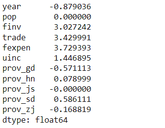
Now we can see that the coefficients of pop and prov_js become 0 because of the penalty by performing L1 regularization in Lasso regression.

(5) Compare prediction results with actual values

Let’s create a comparison table on the model evaluation results using Pandas DataFrame.

actual_pred_compare = pd.DataFrame({'Acutal values':y_test,
'Predicted values':y_test_pred,
'Errors':y_test-y_test_pred,
'MAE':mean_squared_error(y_test, y_test_pred),
'MSE':mean_squared_error(y_test, y_test_pred),
'RMSE':mean_squared_error(y_test, y_test_pred, squared=False),
'MAPE':mean_absolute_percentage_error(y_test, y_test_pred)})
actual_pred_compare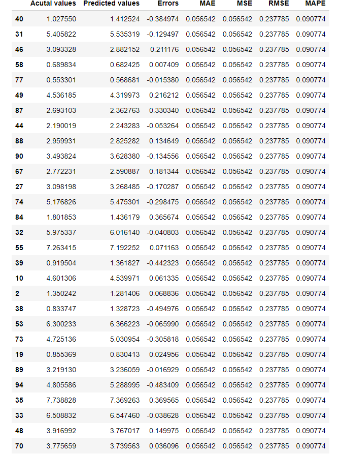

(6) Visualization of the results

Model result visualization is also a helpful way to illustrate the model performance.

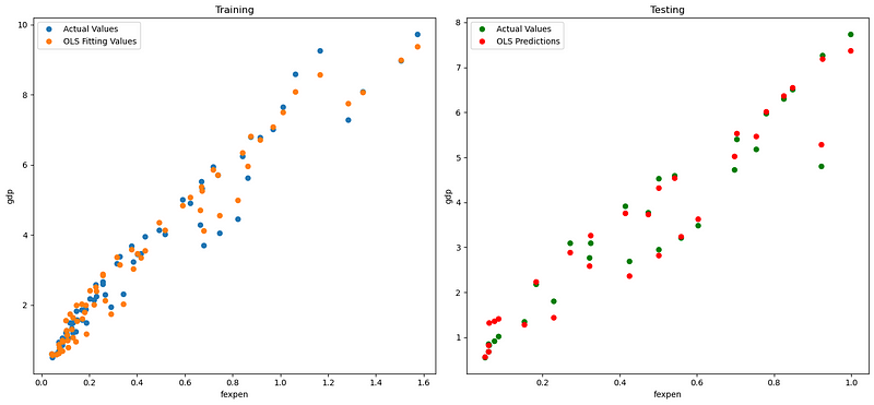
(I) Visualize the fitting and testing results

fig, axes = plt.subplots(1,2,figsize=(15,7))

axes[0].plot(X_train['fexpen'], y_train, "o", label="Actual Values")
axes[0].plot(X_train['fexpen'], pred_train, "o", label="OLS Fitting Values")
axes[0].set(xlabel='fexpen', ylabel='gdp', title='Training')
axes[0].legend(loc="best")

axes[1].plot(X_test['fexpen'], y_test,"go", label="Actual Values")
axes[1].plot(X_test['fexpen'], pred_test,"ro", label="OLS Predictions")
axes[1].set(xlabel='fexpen', ylabel='gdp', title='Testing')
axes[1].legend(loc="best")

plt.tight_layout()

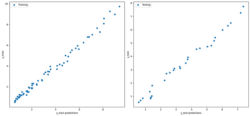
(II) Plot predictions vs. observations

fig, axes = plt.subplots(1,2,figsize=(15,7))

axes[0].plot(y_train_pred, y_train, "o", label="Training")
axes[0].set_xlabel('y_train predictions')
axes[0].set_ylabel('y_train')
axes[0].legend(loc="best")

axes[1].plot(y_test_pred, y_test,"o", label="Testing")
axes[1].set_xlabel('y_test predictions')
axes[1].set_ylabel('y_test')
axes[1].legend(loc="best")

plt.tight_layout()

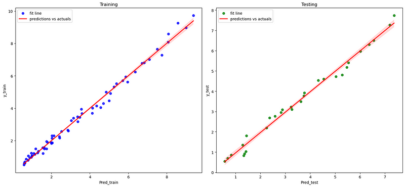
(III) Plot fitting line between predictions vs. observations

fig, axs = plt.subplots(ncols=2,figsize=(15,7))

sns.regplot(x=pred_train, y=y_train,scatter_kws={"color": "blue"}, 
            line_kws={"color": "red"}, ax=axs[0])
axs[0].set(xlabel='Pred_train', ylabel='y_train', title='Training')
axs[0].legend(('fit line', 'predictions vs actuals'),loc=2)

sns.regplot(x=pred_test, y=y_test,scatter_kws={"color": "green"}, 
            line_kws={"color": "red"},ax=axs[1])
axs[1].set(xlabel='Pred_test', ylabel='y_test', title='Testing')
axs[1].legend(('fit line', 'predictions vs actuals'),loc=2)

plt.tight_layout()

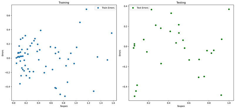
(IV) Plot residuals/errors

fig, axs = plt.subplots(1,2,figsize=(15,7))

axs[0].plot(X_train.fexpen, y_train-pred_train, "o", label="Train Errors")
axs[0].set(xlabel='fexpen', ylabel='Errors', title='Training')
axs[0].legend(loc="best")

axs[1].plot(X_test.fexpen, y_test-pred_test,"go", label="Test Errors")
axs[1].set(xlabel='fexpen', ylabel='Errors', title='Testing')
axs[1].legend(loc="best")

plt.tight_layout()