

Univariate Model for One-Step Ahead Prediction
In this tutorial, we have explored how to use LSTM (Long Short-Term Memory) to predict time series using a real-world dataset apple_share_price.csv. We utilized the Keras library in Python, which provides a convenient API for building and training deep learning models. By following the step-by-step instructions, we have successfully built a simple Univariate LSTM model that can make predictions on time series data.
To begin, we imported the necessary libraries such as pandas, NumPy, and Keras. We then loaded and preprocessed the dataset, ensuring that the time series data was in the appropriate format. We split the dataset into training and testing sets and scaled the data using MinMaxScaler to ensure the LSTM model could work effectively.
Next, we prepared the training data by creating input sequences and target values using a sliding window approach. This allowed the LSTM model to learn patterns and make predictions based on historical data. We then proceeded to build the LSTM model, which consisted of an LSTM layer and a dense output layer. The model was compiled using an appropriate optimizer and loss function.
After building the model, we trained it using the prepared training data and evaluated its performance on the testing set. We calculated the root mean squared error (RMSE) to assess the accuracy of the predictions compared to the actual values.
Finally, we demonstrated how to use the trained LSTM model to make one-step-ahead predictions on future unseen data. By scaling the input data and utilizing the trained model, we obtained predicted values for the future time steps.
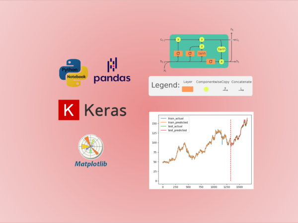
In this tutorial, we will use the Keras library in Python, which provides a convenient API for building and training deep learning models.
Step 1: Import the required libraries
First, let’s import the necessary libraries:
import pandas as pd
import numpy as np
import matplotlib.pyplot as plt
from sklearn.preprocessing import MinMaxScaler
from keras.models import Sequential, load_model
from keras.layers import LSTM, Dense
Step 2: Load and preprocess the dataset
Next, we need to load and preprocess the time series dataset. For this tutorial, let’s use a CSV file named “apple_share_price.csv” containing the historical time series data of Apple share prices. We read it directly from GitHub.
url = 'https://raw.githubusercontent.com/NourozR/Stock-Price-Prediction-LSTM/master/apple_share_price.csv'
df = pd.read_csv(url,usecols=[0,1,2,3,4])
df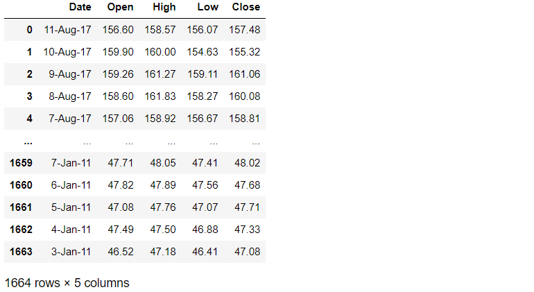
We have discussed how to reverse the order of the rows with 5 different methods in this previous article. You can reverse the rows in chronological order.
df = df.reindex(index = df.index[::-1]).reset_index(drop=True)
df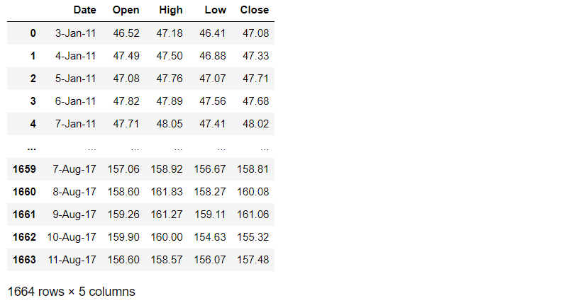
The dataset contains 1664 rows and 5 columns. In this example, we only use the column of ‘Open’.
df= df[['Open']]
df.head()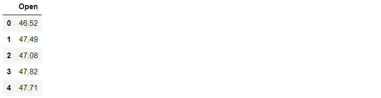
Step 3: Visualize the data
We use Matplotlib to visualize the dataset.
plt.plot(df)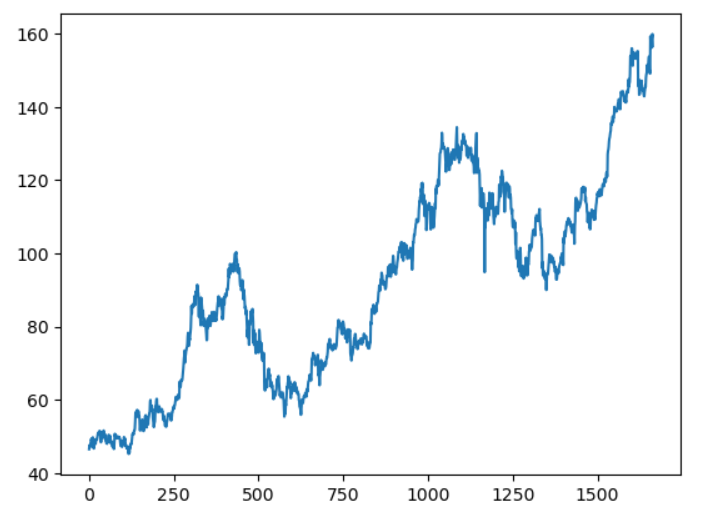
Step 4: Split the dataset into training and testing sets
Before training the LSTM model, we need to split the dataset into a training set and a testing set. Typically, we use a majority of the data for training and a smaller portion for testing. In this tutorial, let’s use 80% of the data for training and 20% for testing:
train_size = int(len(df) * 0.8)
train_data = df.iloc[:train_size]
test_data = df.iloc[train_size:]
Step 5: Scale the data
LSTMs are sensitive to the scale of input data, so it’s important to scale the data before training the model. We can use the MinMaxScaler from scikit-learn to scale the values between 0 and 1:
scaler = MinMaxScaler(feature_range=(0, 1))
train_scaled = scaler.fit_transform(train_data)
test_scaled = scaler.transform(test_data)
Step 6: Prepare the training data
To train an LSTM model, we need to prepare the input sequences and target values. We will create a sliding window of input sequences and their corresponding target values.
def create_sequences(data, input_size):
    X, y = [], []
    for i in range(len(data) - input_size):
        X.append(data[i:i + input_size])
        y.append(data[i + input_size])
    return np.array(X), np.array(y)

input_size = 5
X_train, y_train = create_sequences(train_scaled, input_size)
X_test, y_test = create_sequences(test_scaled, input_size
You can check the shape of training and testing dataset as follows:
print(X_train.shape)
print(X_test.shape)
Step 7: Build the LSTM model
Now, let’s build the LSTM model using Keras. We will create a sequential model with an LSTM layer and a dense output layer:
model = Sequential()
model.add(LSTM(100, activation=’relu’,input_shape=(X_train.shape[1], X_train.shape[2])))
model.add(Dense(1))
model.compile(optimizer=’adam’, loss=’mse’)
Step 8: Train the model
We can now train the LSTM model using the prepared training data:
history = model.fit(X_train, y_train, epochs=50, batch_size=50,validation_split=0.2)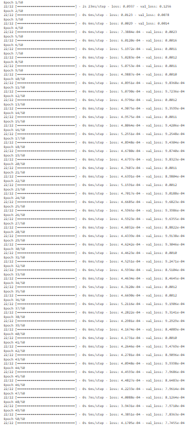
# plot training history
plt.plot(history.history[‘loss’], label=’train’)
plt.plot(history.history[‘val_loss’], label=’validation’)
plt.legend()
plt.show()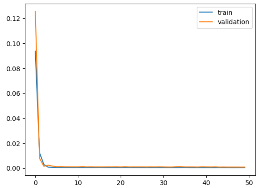
Step 9: Save the Model
We can easily save the trained model, and load it back for future use.
model.save(‘./model/simple_lstm_stock_model’)You can load it as follows when you use it.
# loading model
new_model = load_model(‘./model/simple_lstm_stock_model’)
Step 10: Evaluate the model
After training the model, we can evaluate its performance on the testing set:
train_predicted = model.predict(X_train.reshape(X_train.shape))
test_predicted = model.predict(X_test.reshape(X_test.shape))

train_predicted = scaler.inverse_transform(train_predicted)
test_predicted = scaler.inverse_transform(test_predicted)

train_actual = scaler.inverse_transform(y_train)
test_actual = scaler.inverse_transform(y_test)

train_rmse = np.sqrt(np.mean((train_actual - train_predicted) ** 2))
test_rmse = np.sqrt(np.mean((test_actual - test_predicted) ** 2))

print("Train RMSE:", train_rmse)
print("Test RMSE:", test_rmse)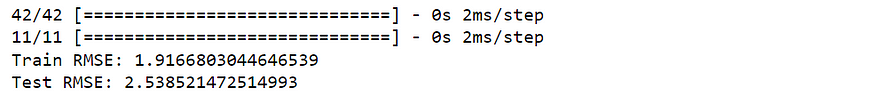
Step 11: Plot the Model Results
We can visualize the training and testing result as follows. First, we create x-axis ranges for train data and test data.
x1 = np.arange(0, len(train_actual))
x2 = np.arange(len(train_actual), len(train_actual)+len(test_actual))
Then you can visualize the actual train data and train fitting results.
plt.plot(x1,train_actual)
plt.plot(x1,train_predicted)
plt.legend(['train_actual','train_predicted'])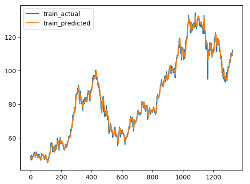
Similarly, you can visualize the model testing result and actual testing data.
plt.plot(x2,test_actual)
plt.plot(x2,test_predicted)
plt.legend(['test_actual','test_predicted'])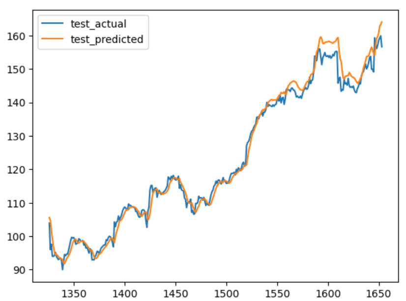
Or you just visualize the training and testing results together. In this example, we use a dashed red line to separate training and testing results. In the previous article, it displays the different methods to plot vertical or horizontal lines.
plt.plot(x1,train_actual)
plt.plot(x1,train_predicted)
plt.plot(x2,test_actual)
plt.plot(x2,test_predicted)
plt.legend(['train_actual','train_predicted','test_actual','test_predicted'])
plt.vlines(x=int(len(train_actual)), color='r',linestyles='dashed', ymin = 0, ymax = max(test_actual))
plt.show()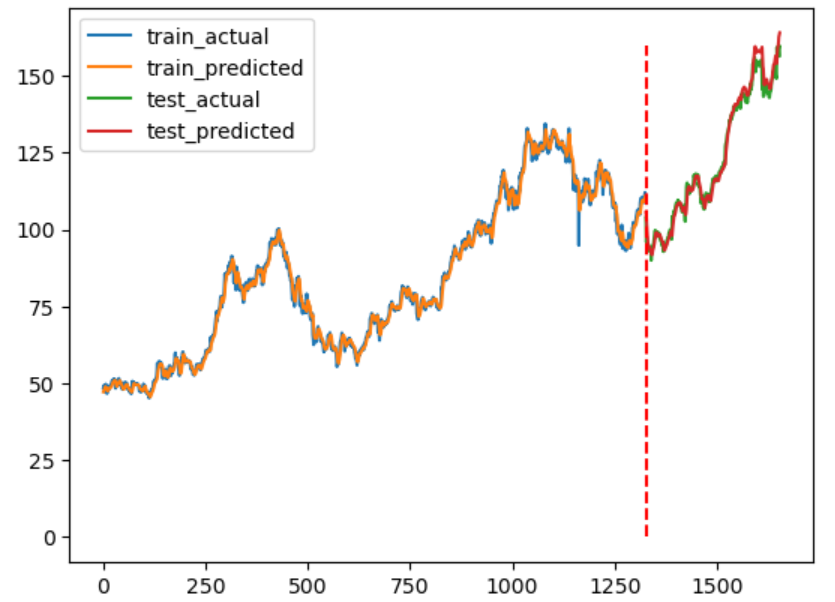
Step 12: Make predictions
Finally, we can use the trained LSTM model to make predictions on future unseen data:
future_data = df.iloc[-input_size:]
future_scaled = scaler.transform(future_data)
future_sequence = np.array([future_scaled])

future_predicted = model.predict(future_sequence)
future_predicted = scaler.inverse_transform(future_predicted)

print("Future predicted values:", future_predicted)
Conclusion
In this tutorial, we have learned how to apply LSTM for time series prediction using a real-world dataset. LSTMs are powerful tools for capturing and learning complex temporal patterns, making them suitable for forecasting future values based on historical data. By following the step-by-step instructions, you have gained hands-on experience in building, training, and evaluating an LSTM model using Keras.
Remember that the performance of the LSTM model can be influenced by various factors such as the size of the sliding window, the number of LSTM units, and the number of training epochs. It’s essential to experiment with different configurations and hyperparameters to optimize the model’s accuracy and generalization.
By mastering LSTM for time series prediction, you can unlock numerous applications in finance, weather forecasting, stock market analysis, and many other domains where understanding and predicting sequential data is crucial. With further exploration and practice, you can continue to refine your skills in building sophisticated deep learning models for time series forecasting.
Originally published at https://medium.com/ on June 24, 2023.