To display decomposition methods of Stationary Wavelet transform (SWT) with PyWavelets using an easily understanding example

In the previous article, we have discussed some key differences, advantages and disadvantages between the Decimated Wavelet Transform (DWT) and the Undecimated Wavelet Transform (UWT). The Stationary Wavelet Transform (SWT) is a powerful signal processing technique that allows the decomposition of a signal into different frequency bands. It has widespread applications in various fields such as image processing, data compression, and denoising.

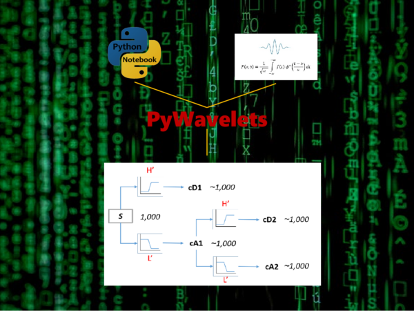
In general, the process of SWT includes the following main steps:

1. Signal Decomposition: The first step in SWT is to decompose the signal into different frequency bands. This is achieved by applying a series of high-pass and low-pass filters to the signal. The high-pass filter extracts the high-frequency components, while the low-pass filter captures the low-frequency components.
2. Filter Banks: SWT utilizes filter banks to perform the signal decomposition. A filter bank consists of a pair of high-pass and low-pass filters that operate simultaneously. The high-pass filter removes the low-frequency components, leaving behind the high-frequency components, while the low-pass filter extracts the low-frequency components.
3. Downsampling: After filtering, downsampling is performed to reduce the sampling rate of the decomposed signals. This step reduces redundancy and facilitates further analysis. Downsampling involves discarding every alternate sample in the signal.
4. Recursive Filtering: SWT involves a recursive filtering process, where the filtering operation is applied repeatedly on the decomposed signals. This recursive filtering creates a multiresolution analysis, allowing the decomposition of the signal into multiple scales.
5. Wavelet Selection: The choice of wavelet function is crucial in SWT. Different wavelets have different characteristics and are suitable for different types of signals. Commonly used wavelets include Daubechies, Haar, and Symlets. The wavelet function determines the properties of the resulting frequency bands.
6. Reconstruction: Once the signal has been decomposed into different frequency bands, it can be reconstructed by performing an inverse SWT. This involves upsampling and applying the inverse filter banks to each scale to obtain the original signal.

In this tutorial, we will explore decomposition methods involved in performing SWT using a concrete and easily understanding example.

1. Decomposition Methods

We’ll use the ‘PyWavelets’ library, which provides convenient implementations of various wavelet transforms, including SWT.

pywt.swt(S, wavelet, level=None, start_level=0, axis=-1, trim_approx=False, norm=False)

Parameters:

• S: Input signal
• wavelet: Wavelet to use (Wavelet object or name)
• level: [int, optional], i.e. the number of decomposition steps to perform
• start_level: [int, optional], The level at which the decomposition will begin (it allows one to skip a given number of transform steps and compute coefficients starting from start_level) (default: 0)
• axis: int, optional Axis over which to compute the SWT. If not given, the last axis is used.
• trim_approx: [bool, optional], If True, approximation coefficients at the final level are retained.
• norm: [bool, optional], If True, transform is normalized so that the energy of the coefficients will be equal to the energy of data. In other words, np.linalg.norm(data.ravel())will equal the norm of the concatenated transform coefficients when ‘trim_approx’ is True.

Returns: coeffs [list] List of approximation and details coefficients pairs in order similar to wavedec function:

[(cAn, cDn), …, (cA2, cD2), (cA1, cD1)]

where n equals input parameter level.

If start_level = m is given, then the beginning m steps are skipped:

[(cAm+n, cDm+n), …, (cAm+1, cDm+1), (cAm, cDm)]

If trim_approx is True, then the output list is exactly as in pywt.wavedec, where the first coefficient in the list is the approximation coefficient at the final level and the rest are the detail coefficients:

[cAn, cDn, …, cD2, cD1]

2. Examples

To illustrate the process, let’s consider a concrete example of analyzing a simple signal using SWT. In this example, we will set different parameters of trim_approx and norm.

(1) trim_approx=False

First, let’s set trim_approx to false, i.e. the default.

import pywt
# create a simple signal
S = [1,2,3,4,5,6,7,7,9,10,11,12,13,14,15,16]
# S = list(range(1,17))

# decompose with SWT
coeffs = pywt.swt(S, 'db2', level=2)
coeffs

[(array([18.19615242, 11.98325318, 7.56490474, 5.9411071 , 7.8161071 ,9.72460075, 11.5080944 , 13.16658805, 15.29158805, 17.39984123,19.30264521, 22. , 26.19615242, 28.39230485, 29.12435565,26.39230485]),
array([-4.92820323, -2.79455081, -0.89174682, 0.51225953, 0.04575318,-0.72876588, -0.35376588, 0.17075318, 0.13725953, 0.10825318,-0.9375 , 0.73205081, 8.92820323, 9.66025404, -2. ,-7.66025404])),
(array([ 8.62398208, 2.31078903, 3.7250026 , 5.13921616, 6.55342972,8.09705281, 9.15771298, 9.95955411, 11.72732106, 13.62449753,15.0387111 , 16.45292466, 17.86713822, 19.28135178, 22.76611771,20.59402938]),
array([-2.07055236e+00, 1.66533454e-16, 1.11022302e-16, 3.33066907e-16,4.44089210e-16, 4.82962913e-01, -8.36516304e-01, 2.24143868e-01,1.29409523e-01, 4.44089210e-16, 8.88178420e-16, 8.88178420e-16,4.44089210e-16, 4.44089210e-16, 7.72740661e+00, -5.65685425e+00]))]

You can extract the approximation and details coefficients as follows.

(cA2, cD2), (cA1, cD1) = coeffs

print('cA2:\n', cA2)
print('cD2:\n',cD2)
print('cA1:\n',cA1)
print('cD1:\n',cD1)

cA2:
 [18.19615242 11.98325318  7.56490474  5.9411071   7.8161071   9.72460075
 11.5080944  13.16658805 15.29158805 17.39984123 19.30264521 22.
 26.19615242 28.39230485 29.12435565 26.39230485]
cD2:
 [-4.92820323 -2.79455081 -0.89174682  0.51225953  0.04575318 -0.72876588
 -0.35376588  0.17075318  0.13725953  0.10825318 -0.9375      0.73205081
  8.92820323  9.66025404 -2.         -7.66025404]
cA1:
 [ 8.62398208  2.31078903  3.7250026   5.13921616  6.55342972  8.09705281
  9.15771298  9.95955411 11.72732106 13.62449753 15.0387111  16.45292466
 17.86713822 19.28135178 22.76611771 20.59402938]
cD1:
 [-2.07055236e+00  1.66533454e-16  1.11022302e-16  3.33066907e-16
  4.44089210e-16  4.82962913e-01 -8.36516304e-01  2.24143868e-01
  1.29409523e-01  4.44089210e-16  8.88178420e-16  8.88178420e-16
  4.44089210e-16  4.44089210e-16  7.72740661e+00 -5.65685425e+00]

In this example, we choose ‘db2’ wavelet and decompose a simple signal into 2 levels using SWT method with the default settings of trim_approx=False and norm=False. We obtain pairs of approximation and detail coefficients at the decomposed levels, i.e. 2 levels in the example.

We check the lengths of the original signal and coefficients.

print(len(S))
print(len(cA2))
print(len(cD2))
print(len(cA1))
print(len(cD1))

16
16
16
16

We see that they have the same length, which results in a shift-invariant wavelet transform. It has been discussed in this point in the previous article.

(2) trim_approx=True

Now we set trim_approx=True and see the results.

coeff2 = pywt.swt(S, 'db2', level=2,trim_approx=True)

coeff2

array([18.19615242, 11.98325318, 7.56490474, 5.9411071 , 7.8161071 ,
9.72460075, 11.5080944 , 13.16658805, 15.29158805, 17.39984123,
19.30264521, 22. , 26.19615242, 28.39230485, 29.12435565,
26.39230485]),
array([-4.92820323, -2.79455081, -0.89174682, 0.51225953, 0.04575318,
-0.72876588, -0.35376588, 0.17075318, 0.13725953, 0.10825318,
-0.9375 , 0.73205081, 8.92820323, 9.66025404, -2. ,
-7.66025404]),
array([-2.07055236e+00, 1.66533454e-16, 1.11022302e-16, 3.33066907e-16,
4.44089210e-16, 4.82962913e-01, -8.36516304e-01, 2.24143868e-01,
1.29409523e-01, 4.44089210e-16, 8.88178420e-16, 8.88178420e-16,
4.44089210e-16, 4.44089210e-16, 7.72740661e+00, -5.65685425e+00])]

Similarly, we extract the approximation and details coefficients, and we also check their lengths.

(trcA2, trcD2, trcD1) =  coeff2

print(trcA2)
print(trcD2)
print(trcD1)
print(len(trcA2))
print(len(trcD2))
print(len(trcD1)

[18.19615242 11.98325318 7.56490474 5.9411071 7.8161071 9.7246007511.5080944 13.16658805 15.29158805 17.39984123 19.30264521 22.26.19615242 28.39230485 29.12435565 26.39230485][-4.92820323 -2.79455081 -0.89174682 0.51225953 0.04575318 -0.72876588-0.35376588 0.17075318 0.13725953 0.10825318 -0.9375 0.732050818.92820323 9.66025404 -2. -7.66025404][-2.07055236e+00 1.66533454e-16 1.11022302e-16 3.33066907e-164.44089210e-16 4.82962913e-01 -8.36516304e-01 2.24143868e-011.29409523e-01 4.44089210e-16 8.88178420e-16 8.88178420e-164.44089210e-16 4.44089210e-16 7.72740661e+00 -5.65685425e+00]
16
16
16

From the above performance, SWT performance with setting trim_approx=True will decompose a signal into the output list exactly as in pywt.wavedec, where the first coefficient in the list is the approximation coefficient at the final level and the rest are the detail coefficients. But the different is that SWT results in the coefficients with the same length as the original signal.

(3) norm=True

Next, we set norm=True and trim_approx=True and see the results.

nocA2, nocD2, nocD1] = pywt.swt(S, 'db2', level=2,trim_approx=True,norm=True)

print(nocA2)
print(nocD2)
print(nocD1)
print(len(nocA2))
print(len(nocD2))
print(len(nocD1)

[ 9.09807621 5.99162659 3.78245237 2.97055355 3.90805355 4.86230038
5.7540472 6.58329403 7.64579403 8.69992061 9.6513226 11.
13.09807621 14.19615242 14.56217783 13.19615242]
[-2.46410162 -1.3972754 -0.44587341 0.25612976 0.02287659 -0.36438294
-0.17688294 0.08537659 0.06862976 0.05412659 -0.46875 0.3660254
4.46410162 4.83012702 -1. -3.83012702]
[-1.46410162e+00 -1.11022302e-16 -1.11022302e-16 -4.99600361e-16
0.00000000e+00 3.41506351e-01 -5.91506351e-01 1.58493649e-01
9.15063509e-02 -2.22044605e-16 -3.33066907e-16 -4.44089210e-16
-2.22044605e-16 -8.88178420e-16 5.46410162e+00 -4.00000000e+00]
16
16
16

As we discussed in Section 1.1., if True, the transform is normalized so that the energy of the coefficients will be equal to the energy of the data.

(4) Comparison

Let’s plot and compare the approximation coefficients decomposed with above SWT methods.

import matplotlib.pyplot as plt

plt.plot(S)
plt.plot(cA2)
plt.plot(trcA2)
plt.plot(nocA2)
plt.legend(['S','cA2','trcA2','nocA2'])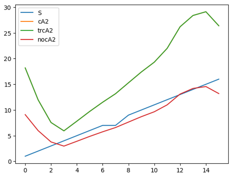

From the visualized comparison, we confirm that approximation coefficient with normalized transform is more closed with the original signal.

Conclusion

The Undecimated Wavelet Transform (UWT) or Stationary Wavelet Transform (SWT) is a powerful signal processing techniqu, which has several advantages over the DWT. This article displays how to decomposition methods using an easily understanding example with Python PyWavelets library. First, we overview the SWT methods, and next we decompose a simple signal into 2 levels with SWT and ‘db2’ wavelet with different parameter settings, such as the default setting, trim_approx=Trueand norm=True.For the normalized transform, the energy of the coefficients will be equal to the energy of data.

Originally published at https://medium.com/  on June 27, 2023.

Please follow and like me: