A Real-World Project of Single-Level Discrete Wavelet Transform of 1D Signal

Discrete wavelet transform using USD-CNY exchange daily time series dataset

We have discussed applications and the basic concepts of wavelet transform, general process and signal extension modes of Discrete Wavelet Transform (DWT) and methods of 1D one stage DWT, and many other topics on Wavelet transform. After you have all this basic knowledge, we move on to a real-world project on single-Level DWT of 1D USD to CNY exchange time series dataset.

1. Introduction to the Project

The objective of this project is to make single-level Discrete wavelet transform (DWT) on a 1D time series signal, which includes the following main tasks:

Make single-level decomposition
Visualize the Approximation and Detail coefficients
Reconstruct the time series signal
Reconstruct the Approximation and Detail
Visualize the Approximation and Detail
Make data noise removal, or noise reduction, or subtraction

2. Prepare Data

(1) Import required packages

We need Pandas to read the dataset and display it in DataFrame, “PyWaveletfor DWTand matplotlib for visualization.

import pandas as pd
import matplotlib.pyplot as plt
import pywt

(2) Read the data

We use historical USD to CNY exchange daily dataset during September 24, 2012 to September 24, 2022. If you use this dataset for other things more than personal study, please cite the dataset source: ca.investing.com, where I downloaded the dataset. For your convenience, I put it in my GitHub repository. You can read the dataset directly from my GitHub repository. If you are not familiar with the method to read dataset from GitHub using Pandas, please read this post.

url = 'https://raw.githubusercontent.com/shoukewei/data/main/data-wpt/USD_CNY%20Historical%20Data.csv'
df = pd.read_csv(url)
df.head()

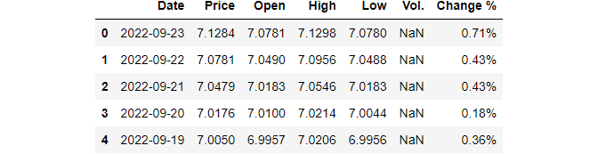
(3) Slice the time and price signal

Suppose we use the Price column as the signal (S) and Data column as the time axis of the signal (t).

t = pd.to_datetime(df["Date"]) 
S = df['Price']

(4) Plot the signal

Now, let’s visualize the signal using matplotlib.

fig, ax = plt.subplots(figsize=(15,5))
ax.plot(t,S)
ax.set_xlabel('t (Day)',fontsize=14)
ax.set_ylabel('Signal (Price)',fontsize=14)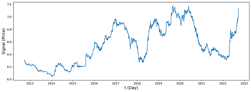

3. Single-level Wavelet Decomposition

In this section, we decompose the signal at the first level using DWT methods, which were discussed in previous posts,

(1) 1D single-level DWT

We use db2 wavelet and sym signal extension model in this project.

(cA,cD) = pywt.dwt(S,'db2','sym')

(2) Print the coefficients

print('Approximation Coefficient: \n',cA)
print('Detail Coefficient: \n',cD)

The results look as follows:

Approximation Coefficient: 
 [10.06329622 10.03529818  9.9410734  ...  8.90362945  8.9165788
8.92294747]
Detail Coefficient: 
 [ 0.03080233 -0.00255284  0.00374649 ...  0.00016898  0.00163954
0.00093243]

(3) Length of the coefficients

We can print the coefficient length using the following method, or the method introduced in the previous post.

print('Length of orignal signal: ',len(s))
print('Length of Approximation Coefficient: ', len(cA))
print('Length of Detail Coefficient: ',len(cD))

The results are:

Length of orignal signal:  2593
Length of Approximation Coefficient:  1298
Length of Detail Coefficient:  1298

4. Visualization of Approximation and Detail Coefficients

We plot the approximation and detail coefficient, and then save the plot in the result folder in the working directory. If you are interested in systematic methods on data visualization, you can start from this post.

fig,axs = plt.subplots(1,2,figsize=(15,5))

plt.rc('xtick',labelsize=15)
plt.rc('ytick',labelsize=15)

axs[0].plot(cA)
axs[0].set_ylabel('1st level Approximation coefficient (cA)',fontsize=15)
axs[0].set_xlabel('t (year)',fontsize=15)

axs[1].plot(cD)
axs[1].set_ylabel('1st level Detail coefficient (cD)',fontsize=15)
axs[1].set_xlabel('t (year)',fontsize=15)

plt.tight_layout()

plt.savefig('./results/approx_detail_coeff_1level.png',dpi=500)

plt.show()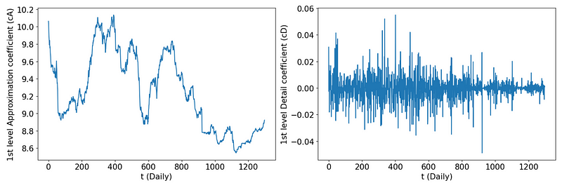

5. Reconstruct the Signal

Here, we use the idwt method to reconstruct the signal.

(1) inverse discrete wavelet transform

S_rec = pywt.idwt(cA,cD,'db2','sym')

(2) Check the lengths

Let’s check if the length of reconstructed signal is the same with original signal. We have discussed that odd length signal will have one more extra value added at the end during DWT in the previous post.

print('Length of orignial signal: ',len(S))
print('Length of reconstructed signal: ',len(S_rec))

The results are:

Length of orignial signal:  2593
Length of reconstructed signal:  2594

(3) Reconstructed signal

As we discussed in the method posts, the final reconstructed signal is the one after removing the last value.

S_rec = S_rec[:-1]

(3) Evaluate the reconstruction

First, we check how well the reconstructed signal presents the original one using visualization method.

# a simple plot
plt.plot(S)
plt.plot(S_rec)

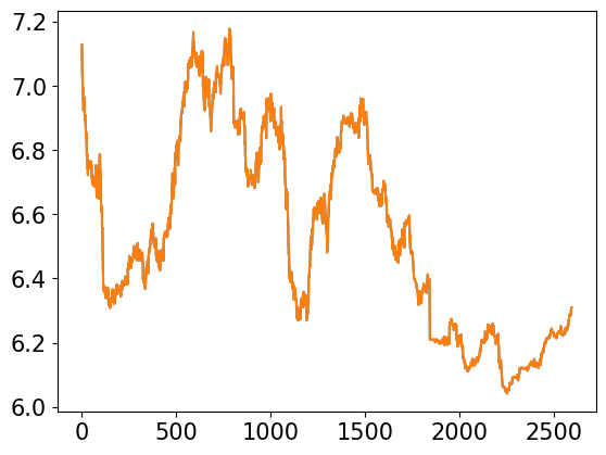
It seems that we cannot the different between the constructed signal and original one. Next, let’s check the reconstruction performance by the Mean absolute error (MAE) and maximum absolute error (Max. AE).

# errors
print('MAE:',sum(abs(S-S_rec))/len(S))
print('Max. AE:'max(abs(S-S_rec)))

The results are:

MAE: 7.463712983133717e-16
Max. AE: 2.6645352591003757e-15

There are very small errors, which can be ignored. It confirms that DWT can well reconstruct the original signal.

6. Partial Wavelet Reconstruction

(1) Reconstruct the approximation and detail

In the method post, we introduced two methods to reconstruct the level 1 approximation and detail (A and D) from the coefficients cA and cD. In this project, we use the idwt method. As we discussed in the method post and previous section, our signal has odd length, so we should remove the last values.

A = pywt.idwt(cA, None,'db2','sym')
D = pywt.idwt(None, cD, 'db2','sym')

A = A[:-1]
D = D[:-1]

(2) Visualization of the approximation and details

fig,(ax1,ax2,ax3) = plt.subplots(3,1,figsize=(15,10))

plt.rc('xtick',labelsize=15)
plt.rc('ytick',labelsize=15)

ax1.plot(t,S)
ax1.set_ylabel('Original price signal (S)',fontsize=15)

ax2.plot(t,A)
ax2.set_ylabel('Approximation of Signal Price(A)',fontsize=15)

ax3.plot(t,D)
ax3.set_ylabel('Detail of Signal Price (D))',fontsize=15)
ax3.set_xlabel('t (year)',fontsize=15)

plt.tight_layout()

plt.savefig('./results/approx_detail_1level.png',dpi=500)

plt.show()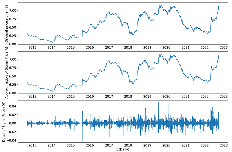

7. Noise Reduction

Detail constituent is the high frequency data, which can be removed as noise. There are some other detailed threshold methods to remove the noise. We just remove the 1st level detail as the noisy in this project. In another way, we just keep the approximation constituent to represent the original signal. Let’s check how well it is.

(1) Visualize approximation vs. original

We visualize the denoised signal (i.e. Approximation in this project) and the orignal signal.

fig,ax = plt.subplots(figsize=(15,6))

plt.rc('xtick',labelsize=15)
plt.rc('ytick',labelsize=15)

ax.plot(t,S)
ax.plot(t,A)
ax.set_ylabel('USD to CNY Exchange Price',fontsize=15)
ax.set_xlabel('t (Daily)',fontsize=15)
ax.legend(('Orignal price signal (s)','Approximation (A)'),loc='best',shadow=True)

plt.savefig('./results/approx_orignal.png',dpi=500)
plt.show()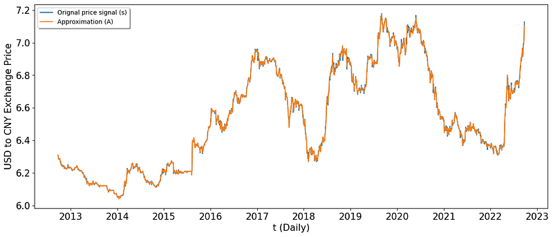

Visualization comparison result illustrates that the approximation can well represent the original signal.

(2) Check errors

Let’s check the erros.

err = sum(abs(S-A))/len(S)
max_err = max(abs(S-A))

print('MAE:',err)
print('Max. AE:',max_err)

The error statistics are:

MAE: 0.004110424877766035
Max. AE: 0.048823329323957054

The errors are very small, which also conforms that the approximation can well represent the original signal.

However, from the denoised point of view, the denoised signal (approximation) is still not so smooth because we only remove the first level details in this project. One-stage DWT is a quick method to make DWT for a signal, but it is suitable for the signal with low frequency. For a high-frequency signal or dataset, a multi-level DWT is needed, and we will talk about this topic in the future.

Online courses

If you are interested in learning how to apply wavelet transform to real-world cases with Python step by step, you are welcome to visit our online school to enroll my courses: