

Master the discrete wavelet decomposition methods using easily understanding examples
The methods for 1D Single-Level Discrete Wavelet Transform in Python will be discussed in the following 3 parts.
(I): Wavelet Decomposition
(II): Wavelet Reconstruction
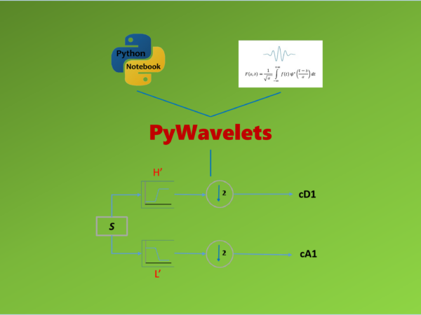
The decomposition process of Discrete wavelet transform (DWT) has been discussed in a previous post. In this tutorial post, we will talk about two concrete methods to decompose a 1D signal into the first level, or one stage using discrete wavelet transform (DWT). For the method parts, simple and easily understanding examples will be used so that we can master the methods quickly, since we can clearly see what results the methods will generate from simple examples. In the future, we will use these methods to solve complicated real-world cases. You will feel everything very easily to understand if you use times to learn these methods here and the concepts of wavelet transform in previous posts.
1. DWT Method
The first method for one stage discrete wavelet decomposition of 1D signal is discrete wavelet transform method (dwt).
(1) DWT method
A single level (or one stage) discrete wavelet decomposition of 1D signal can be easily realized in the PyWavelets using dwt method.
pywt.dwt(signal, wavelet, mode='symmetric', axis=-1)
There are 4 parameters in the function, and it returns approximation and detail coefficients at the first level.
Parameters:
- signal: [array_like] Input signal, or data
- wavelet: [Wavelet object or name] Wavelet to use
- mode: [str, optional] Signal extension mode, see Modes.
- axis: [int, optional] Axis over which to compute the DWT. If not given, the last axis is used.
Returns:
(cA, cD): [tuple] Approximation and detail coefficients
For the signal extension modes, we have already discussed it in the previous post.
(2) An Example
First let’s import the PyWavelets, and next create a simple signal. Then we decompose it.
(i) import pywavelets
import pywt
(ii) create a signal
Here, suppose we have a signal (S) with values only from 0 to 10.
S = [1,2,3,4,5,6,7,8,9,10]
(iii) decompose the signal
Here, we use db2 discrete wavelet and symmetric mode. We have already talked about the built-in wavelet families and members in each family of PyWavelets and signal extension modes in previous posts. If you are not familiar with them, please read them first.
(cA,cD) = pywt.dwt(S,'db2','symmetric')
In many situations, we also use a variable to pack the approximation and detail coefficients. We unpack them when we use each of them.
coeffs = pywt.dwt(S,'db2','symmetric')
(cA, cD) = coeffs
Or we unpacked each of them using:
cA = coeffs[0]
cD = coeffs[1]
(iv) display the decomposed coefficients
Now, we can display the approximation and detail coefficients
print('Approximation Coefficient: \n',cA)
print('Detail Coefficient: \n',cD)
The results look as follows:
Approximation Coefficient:
 [ 1.76776695  2.31078903  5.13921616  7.96764328 10.79607041 13.78858223]
Detail Coefficient:
 [-6.12372436e-01  1.66533454e-16  3.33066907e-16  2.22044605e-16
2.22044605e-16  6.12372436e-01]
2. Downcoef Method
In many cases, however, we probably only care about the approximation coefficient or detail coefficient rather than both of them. This process can be called as Partial decomposition, which is realized using downcoef method.
(1) Downcoef Method
pywt.downcoef(part, data, wavelet, mode='symmetric', level=1)
Parameters:
part: str Coefficients type:
- ‘a’ — approximations coefficient decomposition
- ‘d’ — details coefficient decomposition
data: array_like, Input signal
wavelet: Wavelet name
mode: str, optional. Signal extension mode
level: int, optional. Decomposition level. Default is 1.
Returns:
- coeffs: array of coefficients
(2) An example
We still use the simple signal (S) with values only from 0 to 10 in the above example.
import pywt

# the signal
S = [1,2,3,4,5,6,7,8,9,10]
Suppose we only need the approximation at the first level.
cA = pywt.downcoef('a', S, 'db2', 'symmetric',level=1)
print(cA)
The result is as followsL
[ 1.76776695 2.31078903 5.13921616 7.96764328 10.79607041 13.78858223]
If you require the detail coefficient, you can use the following method.
cD = pywt.downcoef('d', S, 'db2', 'symmetric',level=1)
print(cD)
It produces the following result.
[-6.12372436e-01  1.66533454e-16  3.33066907e-16  2.22044605e-16
2.22044605e-16  6.12372436e-01]
If comparing it with the first method, we find that two methods produce the same results.
3. Calculate Coefficients Length
Length of coefficients arrays are not same, which depend on the selected mode. From the above results of the example, we can clearly see that the lengths of approximation and detail coefficients are both 6. As you know, for a long signal, we can calculate it easily using function len().
We can see or calculate the decompose length easily after we get the decomposition results. But, can we calculate them before decomposition? The answer is ‘yes’?
I would like to introduce the Pywavelets built-in method to calculate them rather than the mathematic equations.
(1) Method
pywt.dwt_coeff_len(data_len, filter_len, mode='symmetric')
Parameters:
- data_len: [int] Data length.
- filter_len: [int] Filter length.
- mode: [str, optional] Signal extension mode
Returns:
len: [int] Length of dwt output.
(2) An example
We still use the simple signal above.
w = pywt.Wavelet(‘db2’)
pywt.dwt_coeff_len(len(S), filter_len=w.dec_len, mode=’symmetric’)
The result will be 6.
You can change the modes, and you will find that periodization mode (per) produces different coefficient length.
w = pywt.Wavelet(‘db2’)
pywt.dwt_coeff_len(len(S), filter_len=w.dec_len, mode=’per’)
The result is 5.