Essentials of Data Visualization with Python Matplotlib (II): the MATLAB-style Interface

Data visualization with Matplotlib is easy with only few lines

The last article generally introduced the plotting libraries in Python, setting up Matplotlib environment, and the process of plotting. In this article, it will focus on how to plot using MATLAB-style Interface.

Matplotlib provides a Matlab-like plotting framework, which allow us to generate a graph in an easy and fast way with only few lines.

Table of Contents

1. Basic Plots

For example, let’s use this interface to draw some basic plots to see how easy it is to use.

First, we should import the module `pyplot`

import matplotlib.pyplot as plt

(1) A Line Plot

Suppose we have a dataset with two variables, x, y, let’s create a simple line plot.

(i) The data

x = [0,1,2,3,4,5,6,7,8,9,10]
y = [0,2,4,3,5,7,6,9,8,10,11]

(ii) Plot the line

plt.plot(x,y)

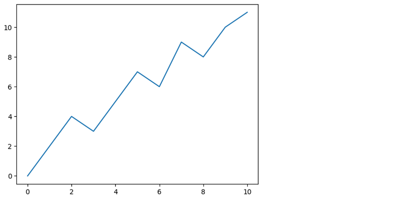
You can see the real plot is only one line.

(iii) Save the figure

plt.savefig('./plots/simpleLine.jpg')

(2) A Bar Plot

Suppose we have a dataset on the average examination scores of each of 7 groups of students, let’s make a bar diagram.

# data
groups = ['Group A', 'Group B', 'Group C','Group D', 'Group E','Group F','Group G']
scores = [80,70,95,60,85,90,98] # examation mean grades for example

# plot bar only in one line
plt.bar(groups, scores)

# Save the figure as .png
plt.savefig('./plots/simpleBar.png')

(3) A Pie Plot

There is a population dataset in a very small town, where there are 20 older people, 40 adults (or young people), 25 children and 15 babies. We make a pie plot and add something a bit interesting, such as exploding the 4th slice (i.e. ‘Babies’), for example.

# Data 
population = 'Olders', 'Alduts', 'Children', 'Babies'
persons = [20, 40, 25, 15]

# plot pie 
explode = (0, 0, 0, 0.1)  # "explode" the 4th slice (i.e. 'Babies')

plt.pie(persons, explode=explode, labels=population, autopct='%1.1f%%',
        shadow=True, startangle=90) # display the percent value using Python string formatting
plt.axis('equal')  # Equal aspect ratio ensures that pie is drawn as a circle.

# save the plot
plt.savefig('./plots/simplePie.png')

(4) A Scatter Plot

Let’s see another widely used plot, scatter plot.

# data
x1 = [0,2,4,3,5,7,6,9,8,10,11]
y1 = [0.1,2.5,3.5,3.8,4.6,7.5,5.6,8.5,10.5,9.5,11.3]

# plot a scatter graph
plt.scatter(x1, y1)

# save the graph
plt.savefig('./plots/simpleScatter.png')

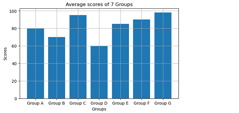
2. Add More Elements

You can add more elements and change features of a plot, such title, x-axis label, y-axis label, legend, grid, font type and size, line types and colors, etc. You can easily add these elements to the plot using the following parameters:

plt.xlabel() set xlable
plt.ylabel() set ylable
plt.title(): gives a tile
plt.xticks(): change xticks, especially font size
plt.yticks(): change yticks, especially font size
plt.legend(): displays the legend
plt.grid(): show grid by setting True

# data
groups = ['Group A', 'Group B', 'Group C','Group D', 'Group E','Group F','Group G']
scores = [80,70,95,60,85,90,98] # examation mean grades for example

# set the size of the plot
plt.figure(figsize=(7, 4))

# plot bar only in one line
plt.bar(groups, scores)

# add more elements
plt.xlabel('Groups')
plt.ylabel('Scores')
plt.title('Average scores of 7 Groups')
plt.grid(True)

# Save the figure as .png
plt.savefig('./plots/averageScoreBar.png')

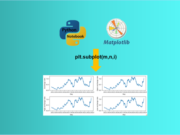
3. Subplot

We usually plot multiple figures, then the subplot method is widely used.

(1) The structure

The structure of the subplot using MATLAB-style Interface in Matlplotlib are very straightforward. I used an example of 2 x 2 subplots to explain the process.

# plot the figure and set its size
plt.figure(figsize=(10, 4))

# create panels and set current axis (rows, columns, panel number)
# for example,subplot 4 graphs with 2 rows and 2 colums

# create the first of 4 panels and set current axis, and then plot
plt.subplot(2, 2, 1) 
plt.plot()

# create the second of 4 panels and set current axis, and then plot
plt.subplot(2, 2, 2)
plt.plot()

# create the third of 4 panels and set current axis, and then plot
plt.subplot(2, 2, 3)
plt.plot()

# create the fourth of 4 panels and set current axis, and then plot
plt.subplot(2, 2, 4)
plt.plot()

# adjust spacing between subplots to minimize the overlaps
plt.tight_layout()

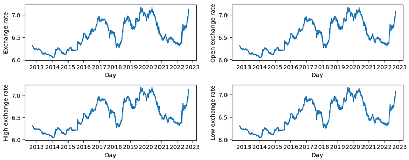
(2) A real example

We will use the USD to CNY exchange daily rate dataset during September 24, 2012 to September 24, 2022. For your convenience, I download this dataset and put it in my GitHub repository. You can download it by clicking this link. If you use this dataset for other things more than personal study, please cite the dataset source: ca.investing.com.

(i) Import required packages and modules

import pandas as pd
import matplotlib.pyplot as plt

(ii) read the data

df = pd.read_csv("./data/USD_CNY Historical Data.csv")

# check the first five data rows
df.head()

(iii) Date conversion

Let’s check the Data to make sure if it is actually a pandas datetime object.

type(df['Date'])

pandas.core.series.Series

The above output shows the Date column is a Series, so you need to transfer it to pandas datetime object if you want it as the x-axis in the plot.

df["Date"] = pd.to_datetime(df["Date"])

(iv) Subplots

We create 4 plots for Price, Open, High and Low using MATLAB-style Interface, and add x-labels and y-labels for each subplot.

# set figure size
plt.figure(figsize=(10, 4))

# create the first of 4 panels and set current axis
plt.subplot(2, 2, 1)
# plot
plt.plot(df['Date'],df['Price'])
# add xlabel and ylabel 
plt.xlabel('Day')
plt.ylabel('Exchange rate')

# create the second of 4 panels and set current axis
plt.subplot(2, 2, 2)
# plot
plt.plot(df['Date'], df['Open'])
# add xlabel and ylabel 
plt.xlabel('Day')
plt.ylabel('Open exchange rate')

# create the third of 4 panels and set current axis
plt.subplot(2, 2, 3)
# plot 
plt.plot(df['Date'], df['High'])  
# add xlabel and ylabel 
plt.xlabel('Day')
plt.ylabel('High exchange rate')

# create the fourth of 4 panels and set current axis
plt.subplot(2, 2, 4)
# plot 
plt.plot(df['Date'], df['Low']) 
# add xlabel and ylabel 
plt.xlabel('Day')
plt.ylabel('Low exchange rate')

# adjust spacing between subplots to minimize the overlaps
plt.tight_layout()

# save the figure
plt.savefig('./plots/USD_CNY_exchange.png')

plt.show()