Develop a Classical Linear Regression Model with Python (III): Model Improvement

A convenient Python function for model improvement by dropping insignificant variables and solve multicollinearity and dummy variables trap

Part I: Model Estimation

Part II: Model Diagnostics

Part III: Model Improvement

Part IV: Model Evaluation

In the previous article, we found the problems existing in the linear regression model, which can be generally summarized as insignificant predictor, multicollinearity, and dummy variables trap. In this article, we see the process to solve these problems first, and then I will display how to use a function that I created to conveniently solve these problems. During the model process, there involves an iterative process of reevaluating the improved model until the final optimal model is obtained.

Table of Contents

1. Stepwise Regression

Stepwise regression is a step-by-step iterative process of removing or adding independent variables in the final model through iteratively examining the statistical significance of each independent variable. There are two stepwise methods, namely forward stepwise and backward stepwise.

Forward stepwise starts to adding an independent variable in the model each time if it is statistical significant. Backward stepwise starts with including all the independent variables to the model as what we have done, and then remove the independent variables that are statistical insignificant one by one until all the rest are significant. It usually starts with removing the one whose p-value is largest if there are several insignificant independent variables. In most case, however, we also check which one to be removed makes the model have smaller error and more accuracy.

In most cases of developing a multiple regression model, there might be many insignificant independent variables. Therefore, it will involve interactive and tedious work. Stepwise regression methods can be helpful for us to choose the significant independent variable easily. There are also some stepwise regression packages in python, which I will not discuss in this post, but probably in a future post. However, stepwise regression can prevent multicollinearity to a great extent, but it is not able to completely solve multicollinearity in most cases. Thus, it is necessary to define a function to solve these two problems in the model.

2. Define the function

The whole function is as follows:

def LRSelect(X_train, y_train, X_train_drop_list):
# drop variables of training dataset
    X_train_drop = X_train.drop(X_train_drop_list,axis=1)
# add constant to the model
    X_train_drop = sm.add_constant(X_train_drop)
# create linear regression model
    model = sm.OLS(y_train, X_train_drop)
    res = model.fit()

# For each X, calculate VIF and save in dataframe
    vif = pd.DataFrame().round(1)
    vif["VIF Factor"] = [variance_inflation_factor(X_train_drop.values, i) for i in range(X_train_drop.shape[1])]
    vif["features"] = X_train_drop.columns

# yield the results
yield X_train_drop
yield res
yield vif

Do not forget to import the required the packages if you use it in a separate python file.

import pandas as pd
import statsmodels.api as sm
from statsmodels.stats.outliers_influence import variance_inflation_factor

The function name is LRSelect, which stands for linear regression select. There are tree parameters:

X_train: the independent variable
y_train: the dependent variable
X_train_drop_list: a list of column names of the independent variables to drop

The first line is to drop the variable(s), which are insignificant or/and have larger VIF. The last three lines use yield statement, which is very similar to return statement. But yield statement returns a generator object to the caller. I use it in code because I want to display the values when we need instead of returning the values directly after calling the function. Other lines in the code snippet were all seen in the previous two posts.

3. Improve the model

Just copy the function in the Jupyter notebook, and run it. Or just download the ModelSelect.py from my GitHub depository, put it in your working directory, and then import it as a module. Here I import as module.

from ModelSelect import LRSelect

(1) Remove the insignificant independent variable(s)

Next, let’s use this function to improve the model we created in the first part, Model Estimation. Based on the results of Model Diagnostics, we know that pop (population) is statistically insignificant, and thus we remove it first.

# remove the pop
X_train_drop_list = ['pop']

# call the function
X_train_drop, res, vif = LRSelect(X_train, y_train, X_train_drop_list)

Then, let’s display the OLS Regression Results by:

res.summary()

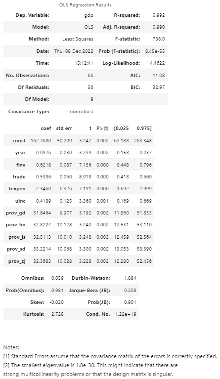
The above results display that the independent variables excluding pop are statistically significant.

(2) Solve multicollinearity

The notes in the above results still indicate that there might be strong multicollinearity. Let’s see VIF to further diagnose it.

vif.round(1)

The results are as follows:

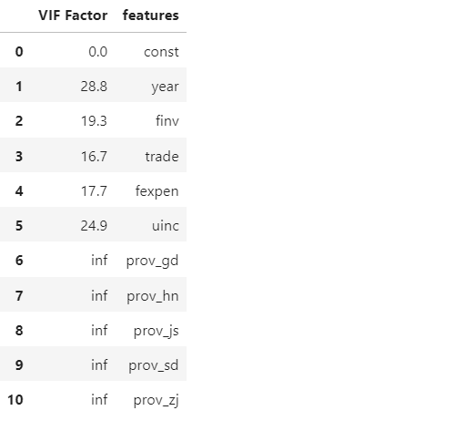
The results further reveal that there are strong multicollinearity. Now, let’s repeat the above process to remove some variables.

(i) Remove one categorical variable

We have already discussed the dummy variable trap problem in the previous post and in another previous post in details. Let’s add prov_gdp in the drop list.

# remove the pop
X_train_drop_list = ['pop','prov_gd']

# call the function
X_train_drop, res, vif = LRSelect(X_train, y_train,X_train_drop_list)

Then check the vif factor to check if there is still multicollinearity.

vif.round(1)

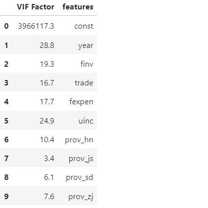
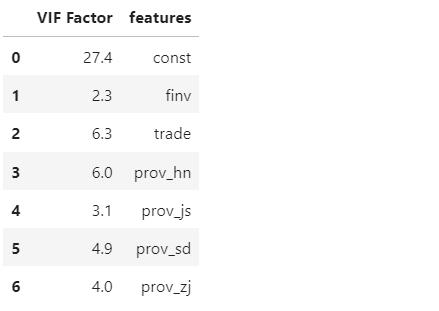
(2) remove other variables with largest VIF one by one

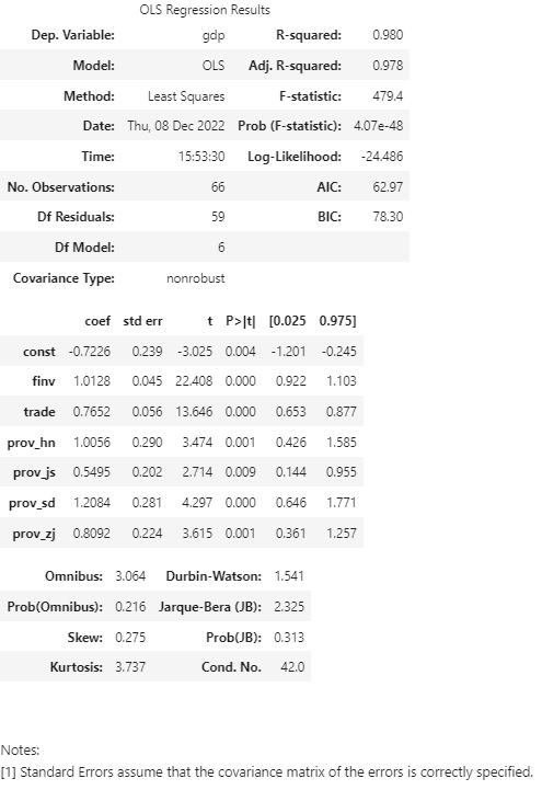
We can see there is still strong multicollinearity. We can repeat the process by removing the variables with the largest VIF one by one. For example, first removing year with VIF of 28.8. If the issue is still there, then remove the largest in the new results. The final results are as follows:

# remove the variables
X_train_drop_list = ['pop','prov_gd','year','fexpen','uinc']

# call the function
X_train_drop, res, vif = LRSelect(X_train, y_train,X_train_drop_list)