Develop a Classical Linear Regression Model with Python (II): Model Diagnostics

Model Diagnostics are an integral part of the model development process, which help us judge whether a model is good or bad

Part I: Model Estimation

Part II: Model Diagnostics

Part III: Model Improvement

Part IV: Model Evaluation

In the previous post, we have created a classical statistic multiple linear regression model. In this article, we will evaluate the model assumptions and check if the model has problems. It is an integral part of the model development process, and the model is usually unbelievable without a reasonable diagnostics evaluation process. In this article, we will see the practical main process of model diagnostics rather than deeply dig into the theory behind.

Table of Contents

1. Model result table

In the last post, we have generated a model result table. I paste this table again as follows so that you need not go backward and forward.

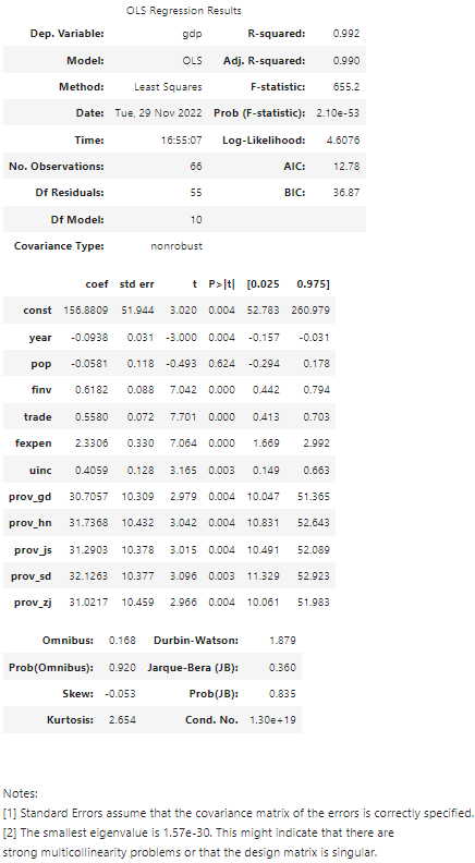
Now, let’s briefly go through these statistics, or metrics.

Df Model: the numbers (N) of predicting variables, i.e. independent variables, minus 1, i.e. N -1. We have 11 independent variables, so DF model is 10 (11–1)
Df Residuals: Degrees of Freedom in the mode. It is calculated in the form of ‘n-k-1’, i.e. ‘numbers of observations — numbers of predicting variables — 1’, that is 66 -11 -1 = 55
Covariance Type: nonrobust. Covariance measures how two variables are linked in a positive or negative manner, and a robust covariance is one calculated in a way to minimize or eliminate variables, here it is not the case.
R-squared (R²): goodness of fit, or determination coefficient. It is interpreted as the proportion of the variance in the dependent variable that is predictable from the independent variable.
Adj. R-squared (Adj. R²): the percentage of variation explained by only the independent variables that actually affect the dependent variable. It will penalize us to add more independent variables which cannot affect the dependent variable. Adjusted R-squared is a modified version of R-squared that has been adjusted for the number of predictors in the model. The adjusted R-squared increases when a new independent variable improves the model, while it decreases when a predictor improves the model by less than expected. Typically, the adjusted R-squared is positive, which is always a bit lower than the R-squared.
F-statistic: assess the significance of the overall model.
Prob (F-statistic) (P-value): If P-value for the F-Stat is less than a significance level, it can reject the null hypothesis and that an intercept-only model is better.
AIC: The Akaike Information Criterion (AIC), which lets us test how well our model fits the data set without overfitting it.
Prob(Omnibus): performs a statistical test indicating the probability that the residuals are normally distributed.
P>|t|: one of the most important statistics in the summary. It is a measurement of how likely the model coefficient is measured through our model by chance.
[0.025 0.975]: the ends of a 95% confidence interval for the parameter.

2. Model Diagnostics

Let’s analyze some most import statistics for evaluating a linear regression model, such R-squared (R²), Adj. R-squared (Adj. R²), Prob (F-statistic) and P>|t| ( p-value).

(1) Goodness of fit

R² is 0.992, which means that the model has very good fitness of the dataset. Adj. R² (0.990) has only very small variation from R², which means that there is no overfitting and the correlation is believable.

(2) Model significance

P-value is very small, indicating that the overall model is statistical significant. Besides, proper model analysis will compare the p-value to a previously established alpha value, or a threshold. The lower the p-value, the more probability it is to reject the null hypothesis, and the greater the statistical significance of the observed difference is.

A common alpha is 0.05. The p value is less than 0.05 is statistically significant. For example, the p value of 0.004 for year means that there is a 0.4% chance the year variable has no effect on the dependent variable, GDP. Whereas, we can see pop (population) does not have a statistically significant relationship with the response variable in the model at the level of 0.05 because its p is 0.624.

(3) Multicollinearity

(i) Multicollinearity issue

Multicollinearity usually occurs in a multiple linear regression model, where two or more independent variables are highly correlated with one another. It means that we can predict an independent variable by another independent variable in a regression model.

Multicollinearity causes the following basic types of problems:

It can increase the variance of the coefficient estimates and make the estimates very sensitive to minor changes in the model.
It reduces the precision of the estimated coefficients, which weakens the statistical power of the regression model. We might not be able to trust the p-values to identify independent variables that are statistically significant.
It also creates an overfitting problem

(ii) Diagnosis methods

There are different methods to assess multicollinearity. One way to assess multicollinearity is to compute the condition number, and values over 20 are worrisome. The statsmodels uses this method in default to test multicollinearity, and this is why the notes on the bottom of the table reveals that the smallest eigenvalue (1.57e-30) might indicate that there are strong multicollinearity problems or that the design matrix is singular.

The specific method to calculate condition number can be referred to: https://www.statsmodels.org/dev/examples/notebooks/generated/ols.html

The second widely used method is to calculate the correlation coefficient matrix or plot a visualized correlation heatmap, which are both talked in a previous post. There exists multicollinearity if two or more predictors are highly correlated with one another. This method is easy and direct. The correlation analysis result in that post indicate that there is multicollinearity due to more variables are highly correlated.

Here, let’s see another widely-used method called VIF (Variance Inflation Factor). It widely accepts that a VIF > 10 as an indicator of multicollinearity, but some scholars choose a more conservative threshold of 5 or even 2.5.

The VIF for each predictor is calculated by creating a linear regression of that predictor on all the other predictors, and next obtaining the R² from that regression. Then VIF for each predictor can be calculated with expression of VIF = 1/(1-R²).

First, we should import this module using:

from statsmodels.stats.outliers_influence import variance_inflation_factor
import statsmodels.api as sm

Then we calculate VIF for each variable and save it into a Pandas DataFrame.

# For each X, calculate VIF and save in dataframe
X_train = sm.add_constant(X_train)
vif = pd.DataFrame()
vif["VIF Factor"] = [variance_inflation_factor(X_train.values, i) for i in range(X_train.shape[1])]
vif["features"] = X_train.columns

vif.round(1)

The result looks as follows:

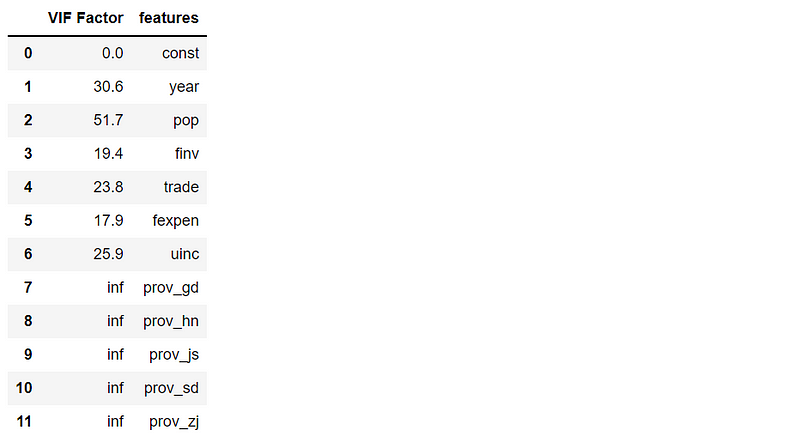
All the VIF factors except the one for constant are larger than 10, which indicate that there are strong multicollinearity problems. Furthermore, VIF factors for the category, dummy or string variables are inf, which mean that regression R² of each these variables are 1, indicating that there is a dummy variable trap. This is why it suggests dropping one column during encoding these variables in that post.

3. Result Summary

The main model diagnostics results shows that: (1) The whole model is statistic significant due to smaller P-value; (2) The model has a very good of fit to the dataset without overfitting due to higher R² (0.992) and Adj. R² (0.990); however, (3) p-value (0.624) for pop (population) reveal that pop does not have statistically significant relationship with the response variable GDP at the significant level of 0.05; however, (4) The condition number, correlation coefficients and Variance Inflation Factors (VIF) all indicate that the model has strong multicollinearity problem; (5) VIF factors for the categorical variables suggest there might be dummy variable trap.