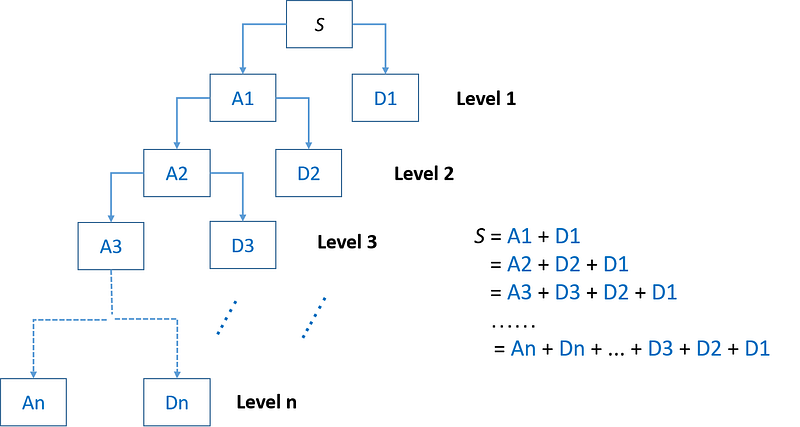


Wavelet partial reconstruction is to reconstruct approximations and details of a signal from their coefficients
Part I: Wavelet Decomposition
Part II: Wavelet Reconstruction
Part III: Wavelet Partial Reconstruction
We have already known what are wavelet decomposition and reconstruction in the previous two parts. In this post, we will talk about the third big part of DWT: general process of partial reconstruction.
1. Wavelet Partial Reconstruction
Partial reconstruction of DWT denotes the process that the real approximations and details of a signal are reconstructed from their approximation coefficients and detail coefficients at different levels.
We will talk about wavelet partial reconstruction from the simple one, i.e. one-stage partial reconstruction because it is much easier to understand. After understanding the one-stage process, the process of multiple stage will be comparatively easier to follow.
2. Single-level Partial Reconstruction
Single-level or one stage partial reconstruction refers to reconstruction the first-level approximation and detail from their approximations and detail coefficient vectors. The process of reconstructing the approximations and details from their coefficient vectors is very similar with the process of reconstructing the signal.
(1) Reconstruct Approximation A1 from the coefficient vector cA1
The coefficient vector cA1 is passed through the same process as reconstructing the signal. Whereas, the difference is that a vector of zeros is feed in place of the detail coefficients vector (cD1). Then, the zero detail coefficients vector (cD1) and the level-one approximation coefficient cA1 are combined to get the approximation.
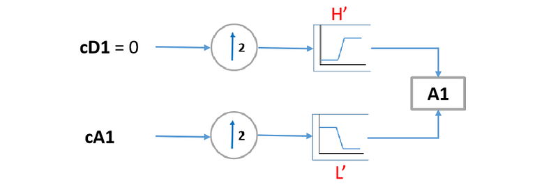
The process yields a reconstructed approximation A1, which is a real approximation of the original signal S and has the same length of it.
(2) Reconstruct the detail D1 from the coefficient vector cD1
The process is similar with reconstruction of the first-level approximation A1. The different is that we feed in a vector of zeros in place of the approximation coefficients vector (cA1) and then combine the zero approximation coefficients vector (cA1) with the level-one detail coefficient cD1.
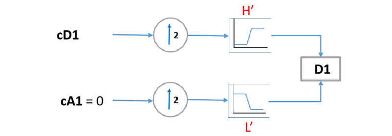
The process yields a reconstructed detail D1, which is a real detail of the original signal S and has the same length of it.
3. Multi-level partial reconstruction
Multi-level partial reconstruction denotes to reconstruct the approximations and details from their decomposition coefficients at different levels.
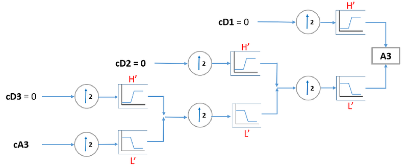
(1) Reconstruct Approximation An from the coefficient vector cAn
The process is to feed in a vector of zeros in place of each of the detail coefficients vector from cDn,…,cD1, and then combine the zero detail coefficients vector (cDn,…, cD1) with the level-one approximation coefficient cA1.
The following diagram is an example of reconstructing approximation A3 from the coefficient vector cA3.
(2) Reconstruct the details (Dn, …, D1) from the coefficient vector (cDn,…,cD1)
Suppose we reconstruct the details at level n (Dn). We feed in a vector of zeros in place of the approximation coefficients vector (cAn), and feed in a vector of zeros in place of each of the detail coefficients vectors at the rest levels except n. Finally, we combine the zero approximation coefficients vector (cAn) and all the zero details coefficients with the detail coefficient cDn.
The following is an example to reconstruct the detail (D3) from its coefficient (cD3).

4. Reconstructing Signal from Approximation and Details
The reconstructed details and approximations are true constituents of the original signal, thus the signal can be reconstructed by summing them.
(1) First Level
For the first level wavelet transform, We can construct the signal by adding the approximation at the first level (A1) and the detail at the first level (D1).

(2) Multi-levels
Extending the one-level technique to the components of a multilevel analysis, it is similar relationships hold for all the reconstructed signal constituents. That is, there are several ways to reassemble the original signal, which can be illustrated using the following tree.