Modelselect: A Python Package Helps Fast Develop Optimal Linear Regression Model

Modelselect package helps get an Optimal Linear Regression Model by removing insignificant variables and solve multicollinearity problems

I developed a small package called modelselect, which can help you fast develop an optimal linear regression model. This is a brief guide to display how to use Python modelselect Package rather than developing a linear regression model. Thus, the process does not strictly follow the modelling processing. If you are interested in linear regression modelling process, please read my previous posts.

Table of Contents

1. Brief Introduction

(1) What is `modelselect`?

A package helps us easily create an optimal linear regression model by removing the insignificant and the multicollinearity predictor variables. This package can reduce the interactive process and tedious work to run the model, estimate it, evaluate it, re-estimate and re-evaluate it, etc. You can find this package on the web of PyPI and GitHub page.

(2) Install the Package

pip install modelselect

(3) Import the Package

from modelselect import LRSelector

then use the LRSelector() directly. Or

import modelselect as ms

then use ms.LRSelector()

(4) Methods

There are three parameters in the functions. modelselect.LRSelector(X, y, X_drop)

Parameters:

X: feature variables, normalized or original
y: target variables
X_drop: a list contains the names of the variables to be removed. The default is empty, i.e. no drop variables

Returns:

res: OLS estimation results
vif: Variance Inflation Factor
X_new: feature variables after removing variables. When X_drop is default, X_new is equal to X.

2. Use Example

(1) Import required packages

Besides this package, we also required numpy,Pandas,statsmodels, normsscaler and scikit-learn. Maybe you are familiar with Pandas, scikit-learn, but you probably do not know normscaler. You can find the normscaler package on PyPi and in one of previous posts.

You can install them using pip as follows if you have not installed them.

pip install pandas, scikit-learn, normscaler

Now, let’s import them as follows.

import numpy as np
import pandas as pd
from statsmodels.tools.eval_measures import meanabs,mse,rmse
import statsmodels.api as sm
from sklearn.model_selection import train_test_split
import modelselect as ms
from normscaler.scaler import DecimalScaler

(2) Read data to Pandas DataFrame

url = 'https://raw.githubusercontent.com/shoukewei/data/main/data-pydm/gdp_china_encoded.csv'
df = pd.read_csv(url,index_col=False)

# display the first rows
df.head()

(3) Define independent variables (X) and dependent variable (y)

GDP is the target and others are features.

X = df.drop(['gdp'],axis=1)
y = df['gdp']

(4) Split dataset for model training and testing

Split the dataset for model training/estimation and testing/validation.

X_train, X_test, y_train, y_test = train_test_split(X, y,test_size=0.30, random_state=1)

(5) Normalize datasets with decimal scaling method

We use the DecimalScaler (Decimal scaling method) in the normscaler package to normalize the X_train and X_test.

X_train_scaled, X_test_scaled = DecimalScaler(X_train,X_test)

(6) Create a linear regression model using `modelselector` package

First, we will use all the feature variables, i.e. there is drop, or X_drop is the default.

modelres = ms.LRSelector(X_train, y_train)

(7) Display the results

(i) display the OLS regression results

res = modelres[0]
res.summary()

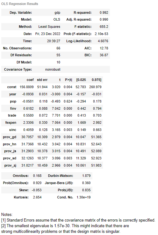
From the above results, we know the model is good, but pop is statistically insignificant at the level of 0.05. There might be strong multicollinearity problems due to the smallest eigenvalue of 1.57e-30.

(ii) display the VIF

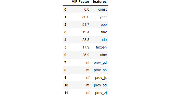
It further confirms that there are strong multicollinearity problems due to the larger VIF. It widely accepts that a VIF > 10 as an indicator of multicollinearity, but some scholars choose a more conservative threshold of 5 or even 2.5.

vif = modelres[1]
vif

(8) Improve the model

First, let’s remove the insignificant variable, pop, and run the model to estimate the model again.

X_drop=['pop']
res_drop_pop, vif_drop_pop,X_drop_pop = ms.LRSelector(X_train, y_train,X_drop=X_drop)

print(res_drop_pop.summary())
print(vif_drop_pop)

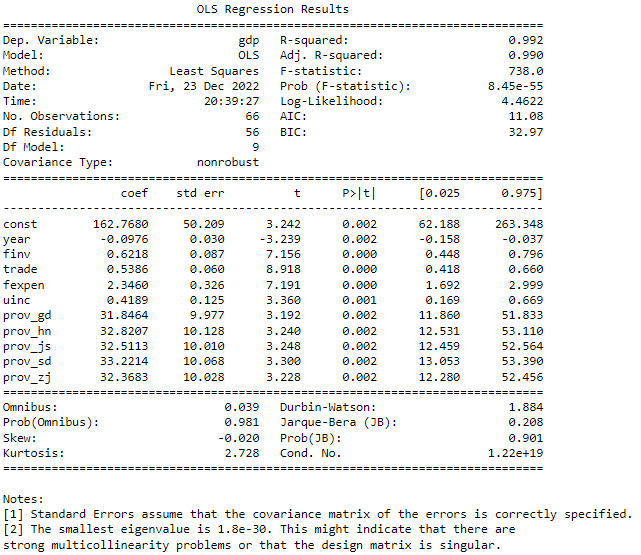
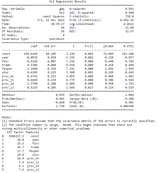
The results display that all the variables after dropping pop are all statistically significant at the level of 0.05. But VIF results shows that the model still has multicollieality.

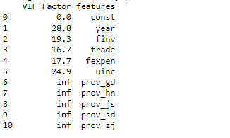
Thus, we need to further drop some variables which VIF is larger than the threshold. Let’s start to drop prov_gd with inf VIF.

X_drop=['pop','prov_gd']
res_drop_gd, vif_drop_gd,X_drop_gd = ms.LRSelector(X_train, y_train,X_drop=X_drop)
print(res_drop_gd.summary())
print(vif_drop_gd)

You can see the VIF of some variables are still larger, then we add the year to the drop list due to its larger VIF. We continue the process untill all the VIFs are less than or equal to 10 except the constant. The final results look as follows.

X_drop=['pop','prov_gd','year','fexpen','uinc']
res_drop_final, vif_drop_final,X_drop_final = ms.LRSelector(X_train, y_train,X_drop=X_drop)
print(res_drop_final.summary())
print(vif_drop_final)

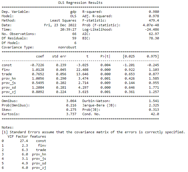
(9) Model validation/testing

Let’s test the model using the testing dataset.

X_test_drop = X_test.drop(['pop','prov_gd','year','fexpen','uinc'],axis=1)

X_test_drop = sm.add_constant(X_test_drop)

y_pred = res_drop_final.predict(X_test_drop)

Then, we calculate MAE, MSE, RMSE and MAPE of the testing.

print("mean_absolute_error(MAE): ", meanabs(y_test,y_pred))
print("mean_squared_error(MSE): ", mse(y_test,y_pred))
print("root_mean_squared_error(RMSE): ",rmse(y_test,y_pred))
print ("mean_absolute_percentage_error(MAPE): ",np.mean((abs(y_test-y_pred))/y_test))

mean_absolute_error(MAE):  0.19150624526331034
mean_squared_error(MSE):  0.05467623605841458
root_mean_squared_error(RMSE):  0.23382950211300238
mean_absolute_percentage_error(MAPE):  0.08418013652994877

The testing results show that the model has very good prediction performance.